One of the most useful features of ML-family languages (OCaml, Standard ML, F# etc) is the type inference. This post contains the notes I took when I was trying to understand the foundational principles of ML type inference.
Damas-Milner Algorithm for Type Inference
Let us take a look at the original type inference algorithm produced
by Damas and Milner. Their language is lambda calculus with
let expression:
e ::= x | λx.e | e e | let x=e in e
Type language composed of a set of type variables (α) and primitive types (ι).
τ = α | ι | τ → τ
σ = τ | ∀α.σ
A Type substitution is [τ1/α1, τ2/α2, ... , τn/αn]. It distinguished
between an α, a type, and α, a type variable.
We define a relation (≥) that relates a more polymorphic type to a less
polymorphic type. For eg, ∀α.α→α ≥ ∀β.β list → β list.
Typing judgment is Γ⊢e:σ.
Instantiation rule is also subtyping rule, where subtyping is defined in terms of “more polymorphic”:
Γ⊢e:σ₁   σ₁≥σ₂
--------------
    Γ⊢e:σ₂
Since there is no explicit big-lambda expression, generalization rule is important:
Γ⊢e:σ  α∈FV(σ)  α∉FV(Γ)
-----------------------
       Γ⊢e:∀α.σ
Basically, ∀α.σ is closure of σ w.r.t Γ (denoted \(\bar{\Gamma}(\sigma)\)).
Let Polymorphism
There is only one rule to introduce polymorphic type into the context Γ:
Γ⊢e:σ       Γ,x:σ⊢e':τ
----------------------
  Γ⊢(let x=e in e'):τ
The Inference Algorithm W:
Uses Robinson’s unification algorithm (U), with following properties:
- U takes a pair of types (τ and τ’), and returns a subtitution V, such that V(τ)=τ’. We say that V unifies τ and τ’
- If substitution S also unifies τ and τ’, then there is another substitution R such that S=R o V.
Algorithm W is shown below:
  Algorithm W

  letrec W(Γ,e) = case e of
    x => let ∀α₁...αn.τ' = Γ(x) in
         let [β₁,...,βn] = freshTyVars(n) in
         let τ = β₁/α₁,...,βn/αn]τ'
             ([],τ)
  | (e₁ e₂) => let (S₁,τ₁) = W(Γ,e₁) in
               let (S₂,τ₂) = W(S₁(Γ),e₂) in
               let β = freshTyVars(1) in
               let V = U(S₂(τ₁), τ₂ → β) in
               let S = V o S₂ o S₁ in
               let τ = V(β) in
                 (S,τ)
  | (λx.e) => let β = freshTyVar(1) in
              let (S₁,τ₁) = W(Γ[x↦β],e₁) in
              let τ = S₁(β)→τ₁ in
                (S₁,τ)
  | (let x=e₁ in e₂) => let (S₁,τ₁) = W(Γ,e₁) in
                        let Γ' = S₁(Γ) in
                        let σ₁ = \bar{Γ'}(τ₁) in (* close τ₁ w.r.t Γ' *)
                        let (S₂,τ₂) = W(S₁(Γ)[x↦σ₁],e₂) in
                        let S = S₂ o S₁ in
                            (S,τ₂)
Observe that substitutions originate only from unification, which happens during function application. A type constraint is solved immediately as it is generated. We accumulate substitutions as we make progress. We apply pending substitutions to Γ before proceeding to next step.
Consider λx.e. We type e under Γ={x:β}, where β is new. Assume e=e₁e₂. Lets say that analyzing e₁ has produced a substitution β ↦ β₁→β₂. Now, before analyzing e₂, we apply this substitution to Γ. That is, we type e₂ under Γ={x:β₁→β₂}. Now, lets say that this yeilded a new substitution β₁ ↦ β₃→β₄. Now, both these substitutions have to be applied to β to determine the type of λx.e.
CONSTRAINT BASED TYPING
Modularity - we separate constraint generation and constraint solving. A separate constraint language can be defined. Can be made as complex as analysis requires.
Constraint-based typing for STLC (Wand,1987):
References:
- T Jones, Type Inference for ML.
- Mitchell Wand, A Simple Algorithm and a Proof for Type Inference, 1987
A Constraint is an equality between two types (i.e., a unification constraint):
datatype C = Eq of τ * τ
The function “constraints” generates a set of constraints to be satisfed for expression e to have type τ under Γ.
constraints : Γ × e × τ → {C}
The function “action” generates top-level constraints that need to be satisfied for e to have type τ under Γ, and a set of type constraints on sub-expressions.
action : Γ × e × τ → {C} × {Γ × e × τ}
The function constraints can be defined in terms of action:
letrec constraints(Γ,e,τ) =
  let bind (s,f) = Set.Union (Set.map s f) in
  let (eqC,tyC) = action (Γ,e,τ) in
  let eqC' = bind(tyC, λ(Γ',e',τ').constraints(Γ',e',τ')) in
eqC ∪ eqC'
Equality constraints can be solved using Robinson’s unification algorithm.
The action function for STLC can be defined as following:
action (Γ,x,τ) = ({τ=Γ(x)}, ∅)
action (Γ,e₁e₂,τ) = let α = freshTyVar() in
      (∅, {(Γ,e₁,α → τ), (Γ,e₂,α)})
action (Γ,λx.e,τ) = let [α₁,α₂] = freshTyVars(2) in
              ({τ=α₁→α₂}, {(Γ[x↦α₁],e,α₂)})
ML Constraint Typing
Since ML has type schemes, to express constraints that arise while analyzing ML expressions, we need a richer constraint language:
C ::= τ=τ' | ∃α₁,...,αn.C | C ∧ C
It is important to remember that the equality in the above constraint
language denotes unification. As such, a less polymorphic type is
unifiable with more polymorphic type. In this sense, perhaps the
unification constraint should be written as τ≤τ'.
We also need a richer type language:
σ ::= τ | ∀{α₁,...,αn | C}.τ
Verification condition is a constraint from above language. It is generated as follows:
Algorithm VC:
letrec VC(Γ,e,τ) = case e of
  c => τ=ty(c)
| x => τ=Γ(x)
| e₁e₂ => ∃α.(VC(Γ,e₁,α→τ) ∧ VC(Γ,e₂,α))
| λx.e => ∃α₁,α₂.(VC(Γ[x↦α₁],e,α₂) ∧ τ=α₁→α₂)
| let x=e₁ in e₂ => VC(Γ[x ↦ ∀{α | VC(Γ,e₁,α)}.α],e₂,τ)
HM(X)
HM(X) itself is parameterized over the constraint domain (X). It makes only a few assumption about language of constraints:
The constraint domain can be
- propositional logic, or first-order logic, in which case the syntax of constraints is same as the syntax of propositional or FOL. The VC generated by HM(x) type inference will be a large conjunction, whose satisfiability (?) yeilds a solution for constraints.
- The domain of syntactic first-order unification problem. The language consists of variables, constants and n-ary uninterpreted functions.
- The domain of semantic first-order unification (i.e., unification modulo theory) problem
The constraint language can also be something, where unification can be reduced to first-order unification.
Aside: Syntax Directed Rules:
When we say a set of rules is syntax directed, we mean:
- There is exactly one rule in the set that applies to each syntactic form, and
- We don’t have to “guess” an input or output for any rule. For eg, To derive a type for e₁e₂, we need to derive types for e₁ and e₂ under same environment.
The initial formulation of type inference algorithm in HM(X) has following properties:
- Constraint normalization (solving) is interleaved with constraint generation. Constraints are normalized as soon as they are generated, yeilding residual constraints and tyvar substitutions as solution.
- The inference algorithm is formulated as a deductive system over clauses of form
ψ,C,Γ ⊢ e:τ, with type environment Γ, expression e as input values, and substitution ψ, constraint C, and type τ as output values. The constraint C captures assumptions over type variables under which the typing holds, and ψ describes type variable substitutions for free variables in Γ.
Following are the rules:
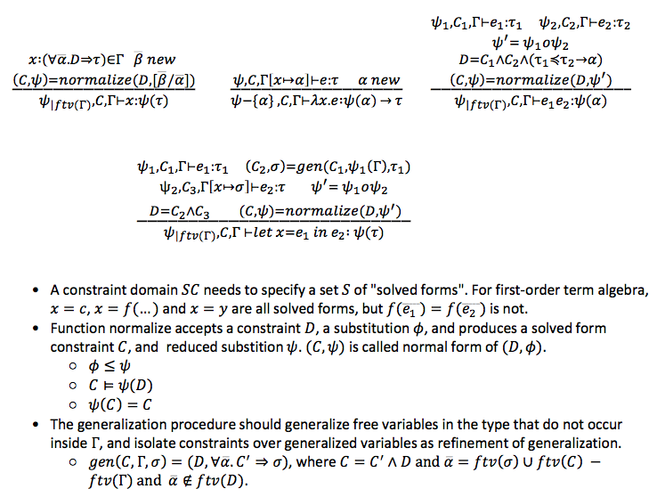
Notes :
- Although constraint generation and constraint solving are interleaved, they are clearly separated. This is unlike the original Damas Milner, where constraints are solved immediately after they are generated, and solution applied globally. Basically, in DM, constraint solving is simple unification, which should be understood as a side-effecting process. In constrast, HM(X) inference keeps collecting constraints, and solves them only when the solution is needed to determine the type of the expression. Constraint solving in HM(X) needs to be more intelligent than unification. It needs something like a worklist algorithm, whereas this process is implicit in case of DM
Example:
fn f => fn x => let y = f x in let z = f (fn v => v) in y
DM (Algorithm W):
- Typechecks top-level let under Γ₁=[f↦α₁, x↦α₂]
- Typechecks f x under Γ₁
- Unifies α₁ with α₂ → β₁, resulting in subst S₁= [α₁ ↦ α₂ → β₁]. Returns S₁ and S₁(β₁) = β₁
- After W over e₁ = f x returns, the substitution S₁ is applied to Γ₁ to yeild Γ₂ = [f↦α₂→β₁, x↦α₂], which is the environment used in the continuation. In further illustration, we capture this process as inplace update of Γ during unification. Type of y is determined to be closure(Γ₂(β₁)) =β₁, as β₁ occurs free in Γ₂.
- Inner let is type checked under Γ₃=Γ₂[y ↦ β₁]. Expression f (fn v => v) is
type checked under Γ₃.
- Unifies α₂→β₁ with (α₃ → α₃) → β₂, resulting in subst S₂ = [α₂ ↦ α₃ → α₃, β₁ ↦ β₂]. This subst is applied globally, leading to Γ₄ = [f ↦ (α₃ → α₃) → β₂, x ↦ α₃ → α₃, y ↦ β₂ ]. The type of the application is β₂.
- The innermost expression y is type checked under Γ₅ = Γ₄[z ↦ closure(Γ₄,β₂)] = Γ₄[z ↦ β₂].
- The type of top-level expression is ((α₃ → α₃) → β₂) → (α₃ → α₃) → β₂
HM(X)
- Typechecks top-level let under Γ₁=[f↦α₁, x↦α₂]
- Typechecks f x under Γ₁
- The constraint generated is [α₁ = α₂ → β₁]. Normalizing (i.e., solving) results in subst S₁= [α₁ ↦ α₂ → β₁]. The type of f x is S₁(β₁) = β₁. (S₁,β₁) is returned.
- After HMX(f x) returns, type (β₁) of y is generalized under Γ₂ = S₁(Γ₁) =
[f↦α₂→β₁, x↦α₂]. It is wrong to generalize it Γ₁, as it erroneously lets β₁ to be generalized, yeilding y:∀β₁.β₁. - However, Inner let is not type checked under Γ₂. It is type checked under
Γ₃ = Γ₁[y ↦ gen(Γ₂,β₁)] = [f↦α₁, x↦α₂, y↦β₁].Expression f (fn v => v) is
type checked under Γ₃.
- The new constraint generated is [α₁ = (α₃ → α₃) → β₂]. Normalizing results in subst S₂ = [α₁ ↦ (α₃ → α₃) → β₂]. The type of the application is S₂(β₂) = β₂. Subst S₂ is also returned.
- After HMX(f (fn v => v)) returns, its type (β₂) is generalized under Γ₄ = S₂(Γ₃) = [f↦(α₃ → α₃) → β₂, x↦α₂, y↦β₁]. No tyvar is generalized.
- The innermost expression y is typechecked under Γ₅ = Γ₃[z ↦ gen(Γ₄,β₂)] = [f↦α₁, x↦α₂, y↦β₁, z ↦ β₂]. The type returned is β₁, and the substitution returned is ∅.
- After both expressions of inner let are type checked, the substitutions are composed and normalized : S₃ = normalize(S₂ o ∅) = normalize(S₂) = normalize([α₁ ↦ (α₃ → α₃) → β₂]) = [α₁ ↦ (α₃ → α₃) → β₂]. The returned result is (S₃,S₃(β₂)) = (S₃,β₂)
- After both expressions of outermost let are type checked, substitutions S₁ and S₃ are composed and normalized : normalize(S₁ o S₃) = normalize ([α₁ ↦ α₂ → β₁, α₁ ↦ (α₃ → α₃) → β₂]). Normalization is essentially constraint solving, which results in following subst: S = [α₁ ↦ (α₃ → α₃) → β₂, α₂ ↦ α₃ → α₃, β₁ ↦ β₂]. The returned result is (S,S(β₂)) = (S,β₂).
- Now, the type of top-level lambda is determined to be S(α₁) → S(α₂) → β₂ = ((α₃ → α₃) → β₂) → (α₃ → α₃) → β₂
Notes
Observe that normalization or constraint solving in HM(X) is tougher than in DM. This is the price we pay for decoupling constraint generation and constraint solving. For constraint generation to be easy, constraint language needs to be expressive so that richer constraints can be expressed. Consequently, solving such constraints becomes tough. If DM is at one extreme, where solving is straightforward unification, at the other extreme is Algorithm VC, shown previously.
Algorithm VC requires expressive constraint language, as shown previously.